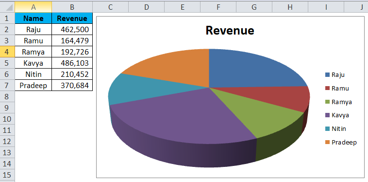
Excel pie chart from list of names
You may learn more about Excel from the following articles Excel. In Excel Click on the Insert tab.
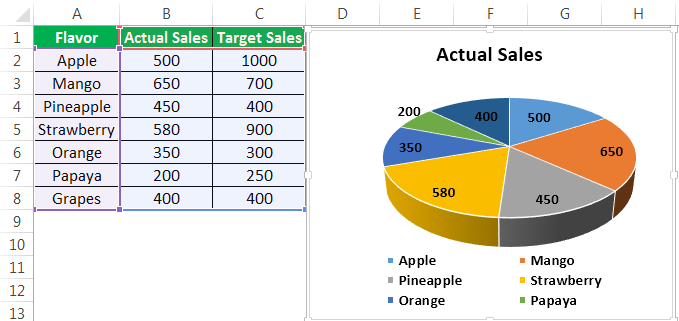
Pie Charts In Excel How To Make With Step By Step Examples
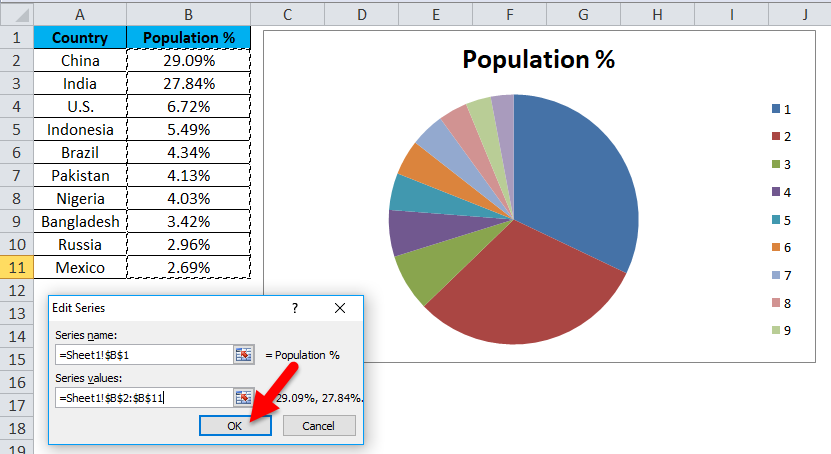
Select the cell range A1B8 go to the Insert tab go to the Charts group click on the Insert Pie or Doughnut.
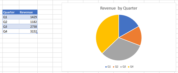
. Enter in the Insert Tab. Follow the below steps to create a Pie of Pie chart. To create a pie chart highlight the data in cells A3 to B6 and follow these directions.
Data thats arranged in one column or row on a worksheet can be plotted in a pie chart. Select Pie of Pie chart in the 2D chart section. Select the chart and click on Chart elements by the top right corner of the chart.
I have chosen 3. Click on the drop-down menu of the pie chart from the list of the charts. In the charts group Select the pie chart button Click on pie chart in 2D chart.
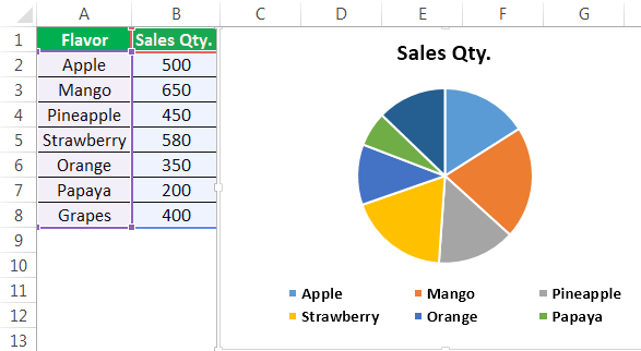
To insert a Pie Chart follow these steps- Select the range of cells A1B7 Go to Insert tab. When laying out your spreadsheet list the names describing. Click on the Insert Tab and.
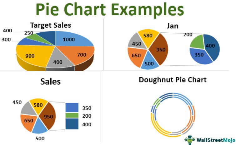
Here we discuss how to make the top five types of pie charts namely 2-D 3-D Pie of Pie Bar of Pie and Doughnut chart. To insert a Pie of Pie chart- Select the data range A1B7. Pie charts show the size of items in one data series proportional to the sum of the items.
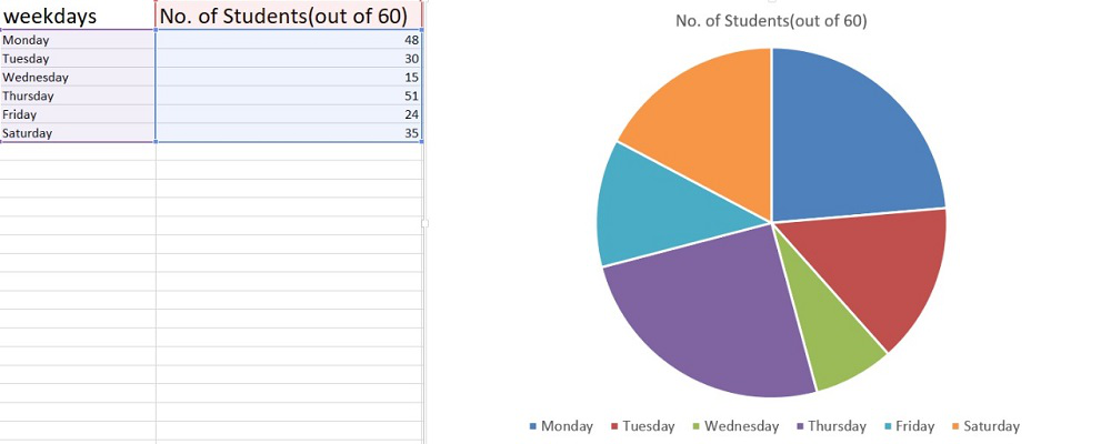
Select the Pie button in the charts group. A pie chart is a percentage chart so only one series of data will be used in the chart. On the ribbon go to the Insert tab.
To create a pie chart highlight the data in cells A3 to B6 and follow these directions. If there is more than one column of data try to list the data to be used in the chart next to the column. Sub SlicesColors Dim chtO As ChartObject Dim ser As Series Dim clf As ColorFormat Dim j As Long loop through all the charts in the worksheet For Each chtO In.
The procedure to create a Bar of Pie Chart for our new data are as follows. Following are some of the steps that can be followed to show legend name in excel. You can choose from a 2-D or 3-D piechart.
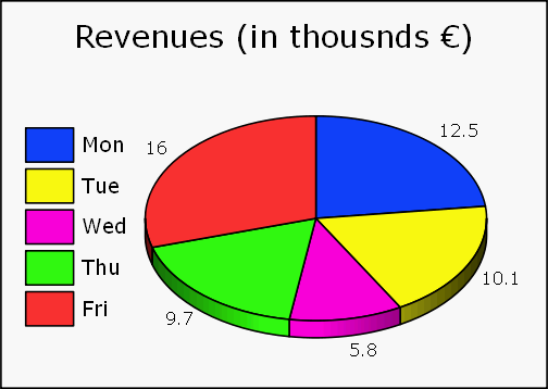
Inserting a Pie Chart Select the cells in the rectangle A23 to B27. Select Insert Pie Chart to display the available pie. Click on the Insert Tab and select Pie from the Charts group.
How To Make A Multilayer Pie Chart In Excel Youtube
Pie Chart In Excel How To Create Pie Chart Step By Step Guide Chart

How To Make A Pie Chart In Excel

Create Multiple Pie Charts In Excel Using Worksheet Data And Vba Pie Charts Pie Chart Pie Chart Template

What Should Your Financial Pie Chart Look Like Pie Chart Financial Budget Financial
Pie Charts In Excel How To Make With Step By Step Examples
Pie Chart In Excel How To Create Pie Chart Step By Step Guide Chart
How To Create A Dynamic Excel Pie Chart Using The Offset Function

Creating Pie Chart And Adding Formatting Data Labels Excel Youtube
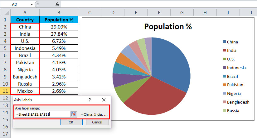
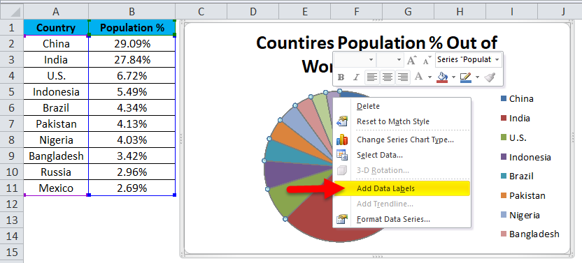
Pie Chart Show Percentage Excel Google Sheets Automate Excel
Pie Chart In Excel How To Create Pie Chart Step By Step Guide Chart
How To Make A Pie Chart In Excel Geeksforgeeks
Pie Chart In Excel How To Create Pie Chart Step By Step Guide Chart
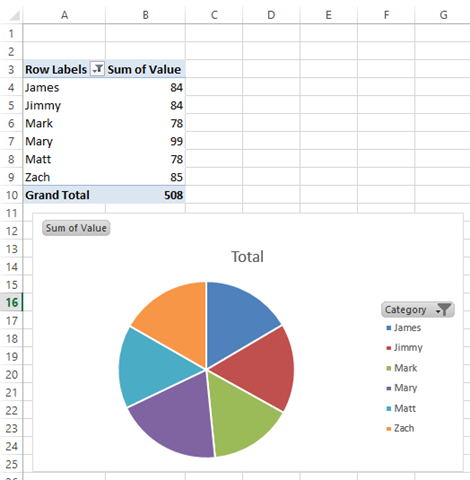
How To Easily Make A Dynamic Pivottable Pie Chart For The Top X Values Excel Dashboard Templates
Pie Charts In Excel How To Make With Step By Step Examples
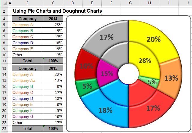
Using Pie Charts And Doughnut Charts In Excel Microsoft Excel 2016

Everything You Need To Know About Pie Chart In Excel